What Is Excel P-Value?
The p-value is used in correlation and regression analysis in Excel, which helps us identify whether the result is feasible and which data set from the result to work with. The value of the p-value ranges from 0 to 1. Unfortunately, Excel has no built-in method to find out the p-value of a given data set. So instead, we use other functions, such as the Chi-Squared test function.
For example, consider the below table showing marks of students obtained in test 1 and test 2. Now, let us learn how to find p-value using T.TEST function.

The steps are:
- Step 1: First, let us find the difference between test 1 and test 2. To do that, we can simply use the formula C2-B2 in cell D2. Press Enter key. We will obtain the difference.
- Step 2: Next, drag using Autofill option till D6 to find the difference.
- Step 3: Now, use the formula =T.TEST(B2:B6,C2:C6,1,1)
We can instantly get the results as shown in the below image.

Likewise, we can use T.TEST function to obtain p-value in Excel.
Key Takeaways
- P-value is used to find if the obtained result is possible to work. It is mostly used in correlation and regression analysis.
- We can change the significance level (alpha value) at different levels and arrive at the p-values in Excel at various points.
- The common alpha values are 0.05 and 0.01.
- If the p-value is >0.10, then the data is not significant. If the p-value is <=0.10, then the data is marginally effective.
- If the p-value is <=0.05, then the data is significant, and if the p-value is <0.05, then the data is highly important.
How To Calculate The P-Value In T-Test In Excel?
Below are examples of Calculating P-Value in the Excel T-Test.
Examples
P-Value Excel T-Test Example #1
In Excel, we can find the p-value easily. By running the T-Test in excel, we can determine whether the null hypothesis is TRUE or FALSE. Look at the below example to understand the concept practically.
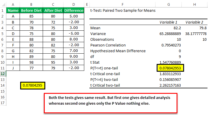
Assume you are supplied with the weight loss process through diet data. Below is the data available to you to test the null hypothesis.
- First, we need to calculate the difference between before and after diet.
The output is given below:Drag the Formula to the rest of the cells.

- Now, go to the “Data” tab, and click on “Data Analysis” under the “Data” tab.

- Now, scroll down and find the “T.Test: Paired Two Sample for Means.”

- Now, we must select “Variable 1 Range” as before the diet column.

- Select “Variable 2 Range” after a diet column.

- The alpha value will be default 0.05, 5% for retaining the same value.
Note:0.05 and 0.01 are often used as common levels of significance.

- Select the “Output Range” where we want to display the analysis results.
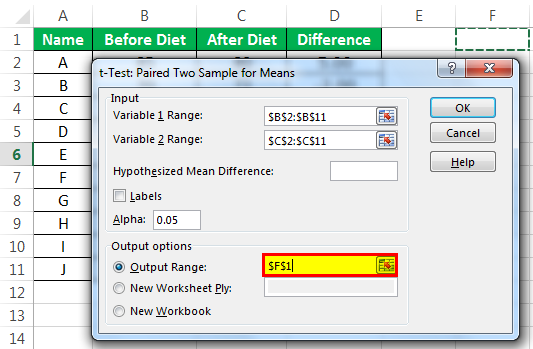
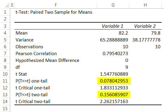
- Click on the “OK.” We have analysis results from cell F1.
We have results here. The p-value with a one-tail test is 0.078043, and the p-value with the two-tail test is 0.156086. In both cases, the p-value is greater than the alpha value, 0.05.In this case, the p-value is greater than the alpha value, so thenull hypothesisis TRUE, i.e., weak evidence against the null hypothesis. It means it is a very close data point between two data points.
P-Value Excel Example #2 – Find P-Value With T.TEST Function
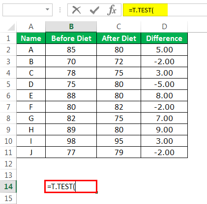
In Excel, we have a built-in function called T.TEST, which can instantly give us the p-value result.
Open the T.TEST function in any of the cells in the spreadsheet.
Select array 1 as before the diet column.

The second argument will be after the diet column, array 2.

Tails will be one-tailed distribution.
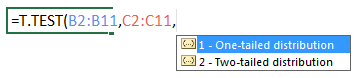
The type will be Paired.

Now, close the formula, and we will have a result of the p-value.

So, we have a p-value of 0.078043, which is the same as the previous test of the analysis result.
Important Things To Note
- P-value is a test used to check if the data we wish to work with is practically possible or not.
- The value of the p-value ranges from 0 to 1.
- There is no in-built method to find the p-value.
- Instead, we can use the T.TEST function.
Frequently Asked Questions (FAQs)
What is p-value in Excel?
The p-value is the probability value expressed in percentage value in hypothesis testing to support or reject the null hypothesis. The p-value or probability value is a popular concept in the statistical world.
Explain the use of p-value in Excel with an example.
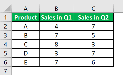
Consider the below table showing sales of various products in Q1 and Q2. Now, let us learn how to find p-value using T.TEST function.
The steps are:
- Step 1: First, let us find the difference between test 1 and test 2. To do that, we can simply use the formula C2-B2 in cell D2. Press Enter key. We will obtain the difference.
- Step 2: Next, drag using Autofill option till D6 to find the difference.
- Step 3: Now, use the formula =T.TEST(B2:B6,C2:C6,1,1)
We can instantly get the results as shown in the below image.

Likewise, we can use T.TEST function to obtain p-value in Excel.
What are the important points to remember while using p-value in Excel?
- Decimal points denote p-value, but it is always good to tell the result of the p-value in percentage instead of decimal points. For example, telling 5% is always better than telling the decimal point 0.05.
- In the test conducted to find the p-value, if the p-value is smaller, the stronger evidence against the null hypothesis and your data is more significant.
- Conversely, if the p-value is higher, there is weak evidence against the null hypothesis. So, by running a hypothesis test and finding the p-value, we can understand the significance of the finding.
Recommended Articles
This article is a guide to P-Value in Excel. We discuss calculating p-value in Excel T-Test, practical examples, and a downloadable Excel template. You may also learn more about Excel from the following articles: –