Conditional Formatting with Formulas - How To Use And Examples.

What Is Conditional Formatting With Formulas In Excel?

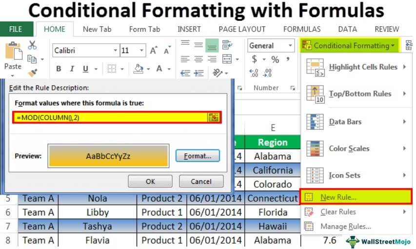
Conditional Formatting with Formula highlights the formula cells based on the condition or criteria given by the user and the received output. We can do that by choosing the “Conditional Formatting” section of the “Home” tab. Then, we click the “New Rule”, and the Conditional Formatting with Formulas option to insert formulas that define the cells to format.

Download FREE Conditional Formatting With Formulas Excel Template and Follow Along!

Download Excel Template

For example, you might have used conditional formatting to highlight the top value in the range and duplicate values. All the formulas should be logical. The result will be either “TRUE” or “FALSE” if the logical test passes, and if the excel logical test fails, we will get nothing.

Key Takeaways

Conditional Formatting with Formulas is a feature mainly used for highlighting the logical results of the set formulas based on the criterias.
We can set simple formulas like greater or less than any values, or use the MOD() function.
It provides a clear distinction between the highlighted cells and the others making the data easy to comprehend and keep track of while working on a large dataset.
Using this feature, we can highlight alternate rows or columns, starting from the first or the second row or column.

Overview Of Conditional Formatting With Formulas

The Conditional Formatting with the formula window with its features, is shown below.

How To Use Excel Conditional Formatting With Formulas?

We can use Excel Conditional Formatting With Formulas in a few methods, namely:

Highlight Cells which has Values Less than 500.
Highlight One Cell Based on Another Cell.
Highlight All the Empty Cells in the Range.
Use AND Function to Highlight Cells.
Use OR Function to Highlight Cells.
Use COUNTIF Function to Highlight Cells.
Highlight Every Alternative Row.
Highlight Every Alternative Column.

Examples

We will consider some examples for Conditional Formatting with Formulas using the above-mentioned methods.

Example #1 – Highlight Cells which has Values Less than 500

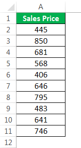
Assume you are working with the sales numbers given below.

Below is the sales price per unit.
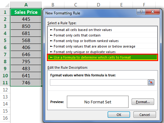
Then, we must go to Conditional Formatting and click on New Rule.
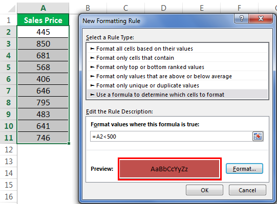
Now, select Use a formula to determine which cells to format.
Now, under Format values where a formula is True, apply the formula =A2<500 and click Format to use theexcel formatting.
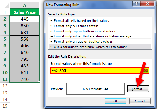
Then, we must select the format as per our choice.
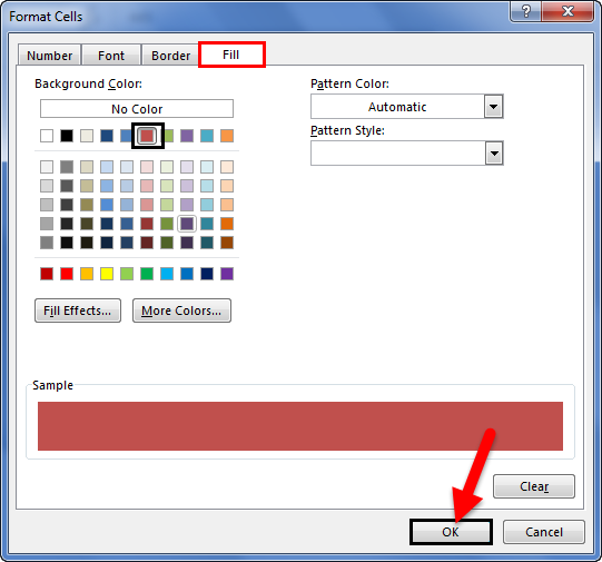
Now, we can see the preview of the format in the preview box.
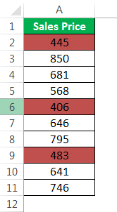
Now, click OK to complete the formatting. As a result, it has highlighted all the cells with a number less than 500, as shown below.

Example #2 – Highlight One Cell Based on Another Cell

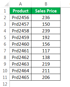
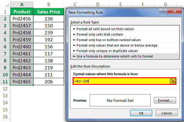
We can highlight one cell based on another cell’s value. For example, assume we have “Product” and “Sales Price” data in the first two columns.

Conditional Formatting Formulas Example 2

The steps to highlight the products from the above table if the sale price is >220 are,

Step 1: First, we must select the “Product” range, go to “Conditional Formatting”, and click on “New Rule”.

Conditional Formatting Formulas Example 2-1

Step 2: In the formula, we must apply the formula as B2 > 220.

Conditional Formatting Formulas Example 2-2

Step 3: Then, click the “Format” key, and apply the format as per choice.

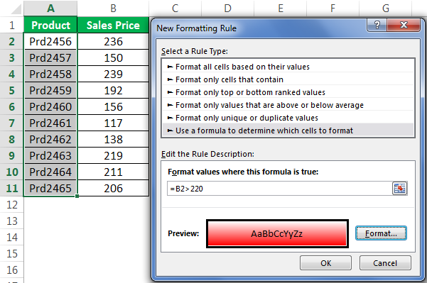
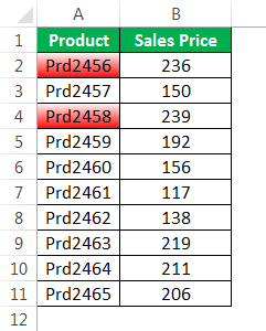
Conditional Formatting Formulas Example 2-3

Step 4: Then click “OK”. Now, we can see that formatting is ready, as shown below.

Conditional Formatting Formulas Example 2-4

Example #3 – Highlight All the Empty Cells in the Range

Assume we have the below-given data.

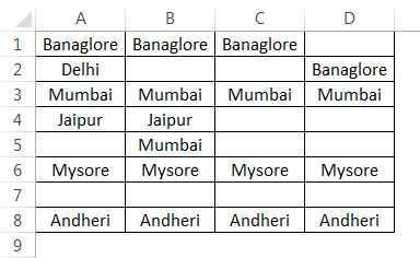
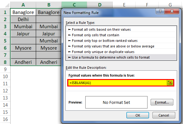
Conditional Formatting Formulas Example 3

We must highlight all the blank or empty cells in the above data because we use the ISBLANK formula in the Excel Conditional Formatting.

Apply the below formula in the formulas section.

Conditional Formatting Formulas Example 3-1

Now, first, we must select the formatting as per our wish.

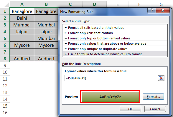
Conditional Formatting Formulas Example 3-2

Click “OK”. It will highlight all the empty cells in the selected range.

Important Things To Note

Conditional Formatting accepts only logical formulas with either “TRUE” or “FALSE” results.
A preview of Conditional Formatting is just an indication of how formatting looks.
We must never use absolute reference as in the formula. When applying the formula, if we select the cell directly, it would make it an absolute reference. We need to make it a relative reference in excel.

Frequently Asked Questions (FAQs)

1. Where is the Conditional Formatting in Excel found?

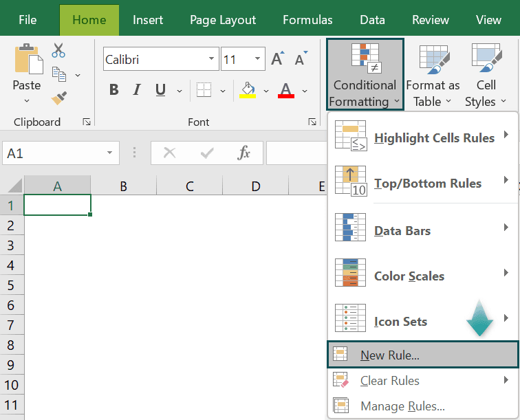
The Conditional Formatting in Excel is found using the following path,

First, choose the dataset → select the “Home” tab → go to the “Styles” group → click the “Conditional Formatting” option drop-down → click the “New Rule” option, as shown below.

Conditional Formatting With Formulas FAQ-1.png

2. Once applied, how can we remove the Conditional Formatting with Formulas in Excel?

We can remove the Conditional Formatting for Formulas as follows:

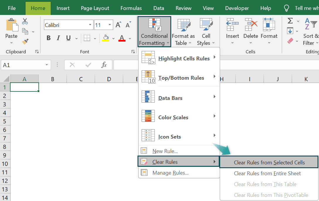
• First, choose the entire dataset or the cell range where the Conditional Formatting Rules are created.
• Next, select the “Home” tab → go to the “Styles” group → click the “Conditional Formatting” option drop-down → click the “Clear rules” option right-arrow → select the “Clear Rules from Selected Cells” option, as shown below.

Conditional Formatting With Formulas FAQ-2.png

Then, all the cells with Conditional Formatting get cleared as it was at the start.

3. Is there an alternative way to copy the Conditional Formatting with Formulas in Excel?

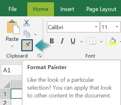
An alternate way to copy the Conditional Formatting Rule is using the “Format Painter”.

• First, select the cells with the Conditional Formatting Rule you want to copy.
• Next, follow the path Home → Clipboard → Format Painter, as shown below.

Conditional Formatting With Formulas FAQ-3.png

• Finally, apply it to the cell value to paste the Conditional Formatting. Then, the font, the color, and every set format will get automatically formatted.