How To Create Dynamic Named Range In Excel? (14 Easy Steps)

What Do You Mean By Excel Dynamic Named Range?

Dynamic named range in Excel is the ranges that change as the data in the range changes, and the dashboard or charts or reports associated with them. So that is why it is called dynamic. So we can name the range from the name box, so the name is a dynamic name range. So, for example, to make a table as a dynamic named range, we must select the “Data,” insert a table and then name the table.

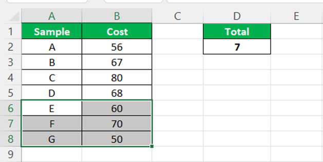
Download FREE Dynamic Named Range Excel Template and Follow Along!

Download Excel Template

For example, consider the below image showing table of samples and cost incurred. The sample size is 4 and it is reflecting in cell D2.

Now, assume that the sample size increases from 4 to 7. Instead of creating new table with formulas, we can readily add the data if we create dynamic named range in Excel as shown in the below image.

Dynamic Named Range in excel Intro Example

Henceforth, dynamic named range in Excel saves time. In this article, let us learn how to create dynamic named range in Excel.

Key Takeaways

Dynamic named range in Excel refers to ranges that change as data in the range changes and the dashboard, charts, or reports associated with them.
To create a dynamic named range, select “Data,” insert a table, and name the table using the name box. This allows for easy customization of the range.
Names should start with a letter, underscore, or backslash, without spaces, and cannot be cell references like A50, B10, or C55.
Excel uses letters C, c, R, and r as selection shortcuts and months and months are treated as identical due to the function’s non-case-sensitive nature.

How To Create Excel Dynamic Named Range? (Step-By-Step)

Dynamic named range in Excel automatically updates the list whenever the data expands. Let us learn how to create dynamic named range in Excel with apt examples.

The steps are:

Now, go to the “Define Name” tab. Give a name to it.

Create data validation for the month list. Select the “List” from the drop-down.

Fill the required details and give a name to define the list.

Now, we must define a new name now under the “Define Name” section.

Give a name to your list and select the range.

Under the “Refers to” section, we must apply the formula as shown in the below image.

Excel dynamically updates the dropdown list when we add additional data.

Rules For Creating Dynamic Named Range In Excel

It will help if we consider certain things while defining the names. But, first, we must follow the below rules from Microsoft, which are pre-determined.

The first letter of the name should begin with a letter or underscore (_) or backslash ()
We cannot give any space in between two words.
We cannot provide a cell reference as our name, for example, A50, B10, C55, etc.
We cannot use letters like C, c, R, and r because Excel uses them as selection shortcuts.

“Define Name” is not case-sensitive. MONTHS and months both are the same.

Examples

Example #1

Consider the below table showing months and data. Let us learn how to create an Excel dynamic named range:

Now, we need to go to the “Define Name” tab.
Click on that and give a name to it.
After that, we must create data validation for the month list.
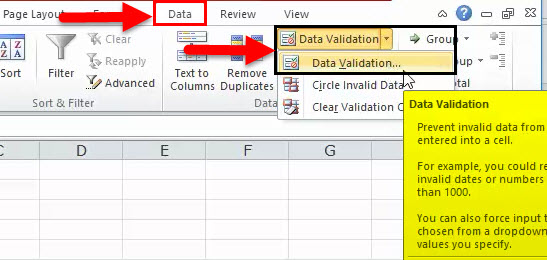
Click on the “Data Validation,” and the below box will open.
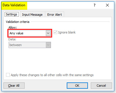
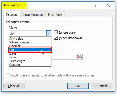
Select the “List” from the drop-down.
Select the”List,” and in “Source, ” we must give the name defined for the month list.
Now, the drop-down list has been created.
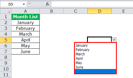
After that, we need to add the remaining six months to the list.
Now, return and check the drop-down list we have created in the previous step. It shows only the first six months. Whatever we have added later, it will not display.
We must define a new name now under the “Define Name” section.
Give a name to your list and select the range.
Under the “Refers to” section, we must apply the formula as shown in the below image.
Now, return and check the drop-down list we have created in the previous step. Now, it shows all the 12 months in the drop-down list. We can see everything in that column.”Name Manager” would dynamically update the dropdown list whenever the data expands.

Example #2

Consider the below table showing inventory of various fruits. Let us learn how to create an Excel dynamic named range.

Now, using OFFSET and COUNTA functions in the Define Name feature, we can make this dynamic.

Next, click on Define Name option – Formulas to open the New Name window. And then, enter a valid name for the range. In this example, let us name it as Inventory.

Next, we enter the formula based on the OFFSET() containing the COUNTA() in the fourth field and click OK to make a dynamic named range in Excel, Experiments.

And then, we need to enter the COUNTA() in the target cell D2.

Likewise, we can create dynamic named ranges in Excel.

Frequently Asked Questions (FAQs)

How to identify all the data in a particular column using Dynamic Named Range in Excel?

To accurately determine the cells containing data, it is essential to identify those that are not empty. The COUNTA function provides a reliable method for counting the number of non-blank cells within a specified range. It is important to note that this function will also include cells with empty strings “”.

For example, consider the below image showing list of participants with their age. The sample size is 3 and it is reflecting in cell D2.

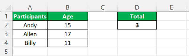
Dynamic Named Range In Excel FAQ 1.png

Now, assume that the sample size increases from 3 to 7. Instead of creating new table with formulas, we can readily add the data if we create dynamic named range in Excel as shown in the below image.

Dynamic Named Range In Excel FAQ 1-1.png

We can use formulas such as COUNTA, OFFSET and/or create a list in Excel. Likewise, we can use dynamic named range in Excel.

How to use Dynamic Named Range in Excel in identifying only numerical data in a particular column?

If you wish to create a dynamic named range that includes a continuous block of solely numeric cells (without any text following the numbers), you can utilize the COUNT function instead of the COUNTA function. In this scenario, the values in column “B” are actually numbers, making the COUNT function more suitable.

How to use Dynamic Named Range in Excel to identify a whole table?

On the ‘Formula’ tab, go to the ‘Defined Names’ group and select ‘Define Name.’ Alternatively, you can press Ctrl+F3 to open the ‘Excel Name Manager’ and click on ‘New.’ In either case, the ‘New Name’ dialogue box will appear, allowing you to enter the necessary details. Once you have entered the details, click ‘OK.’